DCGAN, WGAN and LSGAN: Various interesting network architectures compared

Starting point: DCGAN

As a starting point, I decided to use a DCGAN implementation written in Lasagne for MNIST (source).

I had to modify slightly the generator and discriminator’s network so that they could handle 64×64 colour images. I found the DCGAN to be very unreliable and  it would occasionally manage to learn to generate something that looks like the dataset somewhat only a small fraction of the time. Otherwise, it could spend hundreds or thousands of epochs learning nothing useful.

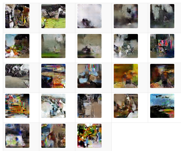
Here is a set of random sample images produced by the generator of the best DCGAN model I trained:

Next model: WGAN

Since the Wasserstein GAN  is reputed to be much more stable under training, I decided to try an implementation. It worked more often than the DCGAN, but still had a high failure rate and was slow to train. Moreover, it had a strange behavior where it would frequently start to learn something for a few hundred epochs and then all of a sudden the critics loss would crash towards 0 in a few epochs and the generator would unlearn everything it had learned and went back to produce garbage.

Problem: limited time and computational resources

In order to save precious time, I implemented a system that would detect when the  critics loss went very low for more than 20 epochs and then abort training. This allowed me to search over a grid of hyperparameters more efficiently.

I did not end up spending much time on WGAN and DCGAN, because I decided to try an even more recent GAN implementation called the LSGAN (Least-Squares GAN). It turned out to produce better results compared to the other 2 implementations.

LSGAN: Best architecture

I tried numerous architectures for the generator and critic’s neural network, but I obtrained the best results with the simplest architecture that I considered, both in terms of training stability and image quality.

Sample images from LSGAN

This is a sample image from my LSGAN. It uses the simplest architecture I tried, with only 3 transpose convolutions.

Issues with the LSGAN generator

As you can see from this sample, there is definitely an issue with image quality and noticeable although not too severe mode collapse.

• Avoiding the checkboard artifacts issue by selecting our transpose convolutions wisely in our generator or by using upsampling via interpolation.
• Feature Matching, perhaps by changing our loss function or adding an additional weighted term which is based on a distance in an intermediate layer of the discriminator (feature maps space instead of pixels space).

There are known solutions to explore and help with the mode collapse, in particular:

• Minibatch Discrimination

This will be attempted if time permits.

Improved sample

Here is a sample image. It was produced with the LSGAN architecture #1 using the following parameters:

• Total training epochs: 1500
• Learning rate eta: 0.0001
• Optimizer: RMSProp
• Batch size: 128
• Sample images produced at epoch: 254

The image contains 100 samples of size 64×64 pixels each, arranged in a 10×10 grid.

Artifacts are still present

Even though this image is a lot smoother, the checkerboard artifact mentioned above is still present in every single image, although not very obvious, it can be seen clearly by zooming in and scaling up one of the images in the sample above:

 

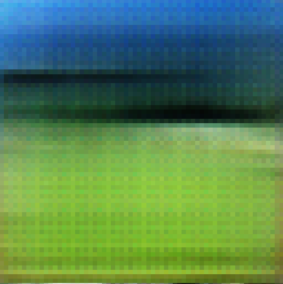
Notice that the checkerboard pattern contains a very high-frequency pattern: the intensity alternates every other pixel. Another pattern can be seen to be repeated every 5 pixels and yet another every 9 pixels.

This phenomenon is caused by the filters of transposed convolutions interfering with themselves in constructive and destructive patterns, as explained in this blog post.

In order to tackle this issue, we replaced every transposed convolution with a regular convolution with stride 1 and “same” padding, in order for the convolution layer to preserve the image dimension. Then, we added an upsampling layer smoothing the scaling output via bilinear interpolation.

Unfortunately, this seems to have severely reduced the capacity of the model and severely reduced the sharpness of the images. Moreover, the checkerboard pattern problem was replaced by a new edges artifact issue, as can be seen in the samples below (one of the best result from this architecture):

To obtain good results from such an architecture, it is therefore probably necessary to increase the neural network’s complexity and therefore its capacity. We attempted doing so, using additional convolution layers, fully-connected layers, greater number of filters, and many other tricks, but they all came with their own set of issues, including a much slower training and a significantly higher probability of total failure to improve during training.